← Back to Math 055

9.1 Euler Methods and Error Analysis: Class Notes

9.1a

Definition

Because Euler’s method, which uses the iterative formula $y_{n+1}=y_n+hf(x_n,y_n)$, $n=0,1,2,\dots$ to approximate solutions to initial-value problems of the form $y\prime =f(x,y)$, $y(x_0)=y_0$, uses approximations, the $y$-values obtained this way contain local truncation error at each step in the approximation.

To determine an upper bound for the size of the error, consider the following. Suppose a function $y(x)$ possesses $k+1$ derivatives that are continuous on an open interval containing $a$ and $x$. The $k^{\text{th}}\text{-degree Taylor polynomial}$ with $\text{remainder}$ for $y(x)$ is

$${\displaystyle y(x)=y(a)+y\prime (a)\frac{x-a}{1!}+\cdots +y^{(k)}(a)\frac{(x-a{)}^k}{k!}+y^{(k+1)}(c)\frac{(x-a{)}^{k+1}}{(k+1)!}}$$

where $c$ is some value between $a$ and $x$. For $k=1$, $a=x_0$, and $x=x_{n+1}=x_n+h$, we have

$${\displaystyle y(x_{n+1})=y(x_n)+y\prime (x_n)\frac{h}{1!}+y″(c)\frac{h^2}{2!}}$$

This is precisely the formula for Euler’s method plus a remainder term. Thus, the local truncation error in $y_{n+1}$ is ${\displaystyle y″(c)\frac{h^2}{2!}}$, where $x_n<c<x_{n+1}$. Since we typically don’t know the value of $c$, an upper bound for the absolute value of the error is $M{h}^2/2$, where $M\ge |y″(x)|$, $x_n<x<x_{n+1}$. We can use the notation $O(h^2)$ to indicate that the magnitude of the error depends on $h^2$. (This is called “big oh” notation, and it essentially indicates that one quantity is bounded by another quantity.)

The first part of the right side is the Taylor polynomial, and the last term is the remainder.

Definition

The total error in approximating $y_{n+1}$ contains local truncation error at each step, and so the result after multiple iterations contains global truncation error.

It can be shown that global truncation error using Euler’s method is $O(h)$.

The improved Euler’s method uses an average of two slopes and has a local truncation error $O(h^3)$ and global truncation error $O(h^2)$.

Improved Euler’s method

First, we use Euler’s method to obtain $y_{n+1}^{*}=y_n+hf(x_n,y_n)$. This is a predictor step.

Then we use ${\displaystyle y_{n+1}=y_n+h\frac{f(x_n,y_n)+f(x_{n+1},y_{n+1}^{*})}{2}}$. This is a corrector step.

Because of the two-step process, this is called a predictor-corrector method.

Euler’s method (from Section 2.6): each step follows the tangent line.

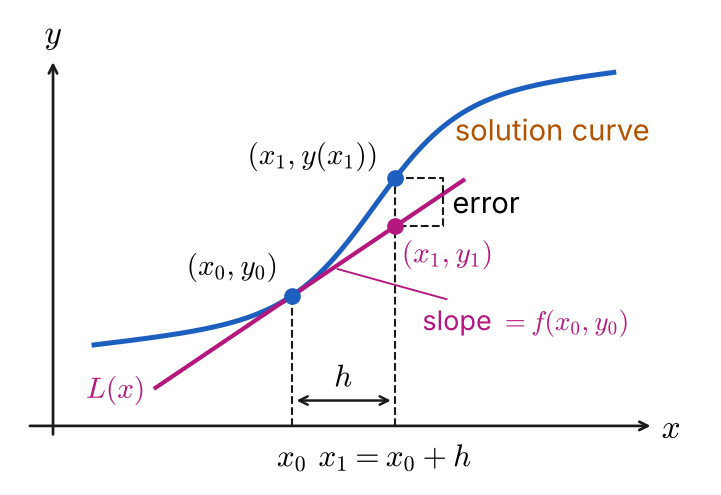
Euler’s method. A solution curve (in blue) passes through $(x_0,y_0)$. The tangent line $L(x)$ at that point has slope $f(x_0,y_0)$. Moving a step $h$ to $x_1=x_0+h$ along the tangent line gives the approximation $(x_1,y_1)$, while the curve itself is at $(x_1,y(x_1))$. The vertical gap between those two points is the error.

Improved Euler’s method: each step follows a line whose slope is the average of two slopes.

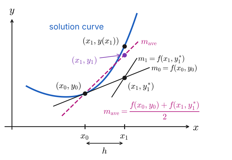
Improved Euler’s method. From $(x_0,y_0)$ on the solution curve, the tangent line with slope $m_0=f(x_0,y_0)$ predicts the point $(x_1,y_1^{*})$. A short line through that point has slope $m_1=f(x_1,y_1^{*})$. The dashed line from $(x_0,y_0)$ has the average slope ${\displaystyle m_{\mathrm{a}\mathrm{v}\mathrm{e}}=\frac{f(x_0,y_0)+f(x_1,y_1^{*})}{2}}$ and gives the corrected point $(x_1,y_1)$, much closer to the curve’s point $(x_1,y(x_1))$ than the prediction.

9.1b

Example

Use the improved Euler’s method to obtain a four-decimal approximation of the indicated value. First use $h=0.1$ and then use $h=0.05$.

$$y\prime =4x-2y,y(0)=2;y(0.5)$$

Solution

$h=0.1$: start with $x_0=0$ and $y_0=2$. Predictor:

$$\begin{array}{cc}\hfill {\displaystyle y_1^{*}}& {\displaystyle =y_0+hf(x_0,y_0)=2+0.1(4(0)-2(2))}\hfill \\ \hfill {\displaystyle }& {\displaystyle =1.6}\hfill \end{array}$$

Corrector, with $x_1=0.1$ and the predicted value $y_1^{*}=1.6$ used in the second slope $f(x_1,y_1^{*})$:

$${\displaystyle \begin{array}{cc}\hfill {\displaystyle y_1}& {\displaystyle =y_0+\frac{h}{2}[f(x_0,y_0)+f(x_1,y_1^{*})]}\hfill \\ \hfill {\displaystyle }& {\displaystyle =2+\frac{0.1}{2}[4(0)-2(2)+4(0.1)-2(1.6)]}\hfill \\ \hfill {\displaystyle }& {\displaystyle =1.66}\hfill \end{array}}$$

Then the next predictor starts from $y_1=1.66$, and gives $y_2$ the same way:

$$y_2^{*}=1.66+0.1(4(0.1)-2(1.66))=1.368\Rightarrow y_2$$

Continuing in a spreadsheet (each row uses $y_n$ to predict $y_{n+1}^{*}$, and the next row’s $y_{n+1}$ uses both slopes):

Compare with the actual values from the analytic solution $y=3e^{-2x}+2x-1$ (found below):

Note that $h\to \frac{1}{2}h$ makes the error about $\frac{1}{4}$ as large: at $x=0.5$, the absolute error drops from $0.0085812$ to $0.0019846$ (and the relative error from $0.78\%$ to $0.18\%$). The error is $O(h^2)$.

Analytic solution: $y\prime +2y=4x$, $y(0)=2$.

Tip: The equation is linear, so an integrating factor $\mu$ works, as do the auxiliary equation (with undetermined coefficients) and Laplace transforms. Two of these are shown.

Using the auxiliary equation, $m=-2$, so $y_c=c{e}^{-2x}$. Try $y_p=Ax+B$, so $y_p\prime =A$:

$$\begin{array}{cc}\hfill {\displaystyle A+2Ax+2B}& {\displaystyle =4x\Rightarrow A=2,B=-1}\hfill \\ \hfill {\displaystyle y}& {\displaystyle =c{e}^{-2x}+2x-1}\hfill \\ \hfill {\displaystyle y(0)=2\Rightarrow 2}& {\displaystyle =c-1\Rightarrow c=3}\hfill \end{array}$$

Or, with the integrating factor $\mu =e^{2x}$:

$${\displaystyle \begin{array}{cc}\hfill {\displaystyle \frac{d}{dx}\left(e^{2x}y\right)}& {\displaystyle =4x{e}^{2x}}\hfill \\ \hfill {\displaystyle e^{2x}y}& {\displaystyle =2x{e}^{2x}-e^{2x}+c}\hfill \\ \hfill {\displaystyle y}& {\displaystyle =2x-1+c{e}^{-2x}}\hfill \end{array}}$$

and $y(0)=2$ again gives $c=3$.