← Back to Math 055

7.1 Definition of the Laplace Transform: Class Notes

7.1a

The Laplace transform is a tool for solving differential equations.

Definition

A transform transforms one function to another function.

Examples of transforms

The derivative and the integral:

${\displaystyle \frac{d}{dx}({\tan }^{-1}x)=\frac{1}{1+x^2}}$ and ${\displaystyle \frac{d}{dx}(x^3)=3x^2}$ are transforms.

${\displaystyle \int \frac{1}{x}dx=\ln |x|+C}$ is a transform.

Transforms possess the linearity properties, e.g.,

$${\displaystyle \frac{d}{dx}[af(x)+bg(x)]=a\frac{d}{dx}[f(x)]+b\frac{d}{dx}[g(x)]}$$

A constant multiple comes out in front of the transform, and a sum is transformed term by term.

Definition 7.1.1

Let $f(t)$ be a function defined for $t\ge 0$. Then the integral ${\displaystyle ℒ\{f(t)\}={\int }_0^{\infty }{e}^{-st}f(t)dt}$ is said to be the Laplace transform of $f$, provided that the integral converges.

The factor $e^{-st}$ is part of the definition; it is always there. The function $f(t)$ is what is being transformed.

The Laplace transform possesses the linearity properties.

Example 1

Evaluate $ℒ\left\{1\right\}$.

Solution

$${\displaystyle \begin{array}{cc}\hfill {\displaystyle ℒ\left\{1\right\}}& {\displaystyle ={\int }_0^{\infty }{e}^{-st}·1dt}\hfill \\ \hfill {\displaystyle }& {\displaystyle ={-\frac{1}{s}{e}^{-st}|}_0^{\infty }}\hfill \\ \hfill {\displaystyle }& {\displaystyle ={-\frac{1}{s{e}^{st}}|}_0^{\infty }=\frac{1}{s},s>0}\hfill \end{array}}$$

For $s>0$, $e^{st}\to \infty$ as $t\to \infty$, so the value at the upper limit is 0. Only the lower limit contributes: ${\displaystyle 0-(-\frac{1}{s})=\frac{1}{s}}$.

Example 2

Evaluate $ℒ\left\{t\right\}$.

Solution

$${\displaystyle ℒ\left\{t\right\}={\int }_0^{\infty }{e}^{-st}·tdt}$$

Integrate by parts with $u=t,dv=e^{-st}dt$, so ${\displaystyle du=dt,v=-\frac{1}{s}{e}^{-st}}$.

$${\displaystyle \begin{array}{cc}\hfill {\displaystyle ℒ\left\{t\right\}}& {\displaystyle ={-\frac{t}{s}{e}^{-st}|}_0^{\infty }+{\int }_0^{\infty }\frac{1}{s}{e}^{-st}dt}\hfill \\ \hfill {\displaystyle }& {\displaystyle ={-\frac{1}{s^2{e}^{st}}|}_0^{\infty }=\frac{1}{s^2}}\hfill \end{array}}$$

The first term is 0: written as ${\displaystyle \frac{t}{s{e}^{st}}}$, the exponential $e^{st}$ grows much faster than $t$, so the term goes to 0 as $t\to \infty$, and it is 0 at $t=0$. This holds for $s>0$.

Example

Evaluate $ℒ\{4t-7\}$

Solution

Using the linearity property, we have

$${\displaystyle ℒ\{4t-7\}=4ℒ\left\{t\right\}-7ℒ\left\{1\right\}=\frac{4}{s^2}-\frac{7}{s}}$$

7.1b

Example

Evaluate $ℒ\{\sin kt\}$

Solution

$${\displaystyle ℒ\{\sin kt\}={\int }_0^{\infty }{e}^{-st}\sin ktdt=I}$$

Integrate by parts with $u=\sin kt,dv=e^{-st}dt$, so ${\displaystyle du=k\cos ktdt,v=-\frac{1}{s}{e}^{-st}}$.

$${\displaystyle I={-\frac{1}{s}{e}^{-st}\sin kt|}_0^{\infty }+{\int }_0^{\infty }\frac{k}{s}{e}^{-st}\cos ktdt}$$

The first term is 0: as $t\to \infty$, $e^{-st}\to 0$ (and $\sin kt$ stays between −1 and 1), and at $t=0$, $\sin 0=0$. Integrate by parts again:

Integrate by parts with ${\displaystyle u=\frac{k}{s}\cos kt,dv=e^{-st}dt}$, so ${\displaystyle du=-\frac{k^2}{s}\sin ktdt,v=-\frac{1}{s}{e}^{-st}}$.

$${\displaystyle I={-\frac{k}{s^2}{e}^{-st}\cos kt|}_0^{\infty }-\frac{k^2}{s^2}{\int }_0^{\infty }{e}^{-st}\sin ktdt}$$

At the upper limit the first term is 0; at the lower limit it is ${\displaystyle -\frac{k}{s^2}}$, so the first term is ${\displaystyle \frac{k}{s^2}}$. The integral that remains is $I$ again:

$${\displaystyle \begin{array}{cc}\hfill {\displaystyle I}& {\displaystyle =\frac{k}{s^2}-\frac{k^2}{s^2}I}\hfill \\ \hfill {\displaystyle (\frac{k^2}{s^2}+1)I}& {\displaystyle =\frac{k}{s^2}}\hfill \\ \hfill {\displaystyle \frac{k^2+s^2}{s^2}I}& {\displaystyle =\frac{k}{s^2}}\hfill \\ \hfill {\displaystyle I}& {\displaystyle =\frac{k}{s^2+k^2}}\hfill \end{array}}$$

Theorem 7.1.1: Transforms of Some Basic Functions

• (a) ${\displaystyle ℒ\left\{1\right\}=\frac{1}{s}}$
• (b) ${\displaystyle ℒ\left\{t^n\right\}=\frac{n!}{s^{n+1}}}$, $n=1,2,3,\dots$
• (c) ${\displaystyle ℒ\left\{e^{at}\right\}=\frac{1}{s-a}}$
• (d) ${\displaystyle ℒ\{\sin kt\}=\frac{k}{s^2+k^2}}$
• (e) ${\displaystyle ℒ\{\cos kt\}=\frac{s}{s^2+k^2}}$
• (f) ${\displaystyle ℒ\{\sinh kt\}=\frac{k}{s^2-k^2}}$
• (g) ${\displaystyle ℒ\{\cosh kt\}=\frac{s}{s^2-k^2}}$

7.1c

Definition

A function $f$ is said to be of exponential order if there exist constants $c,M>0$, and $T>0$ such that $|f(t)|\le M{e}^{ct}$ for all $t>T$.

In words: $f$ does not grow faster than an exponential in the long run.

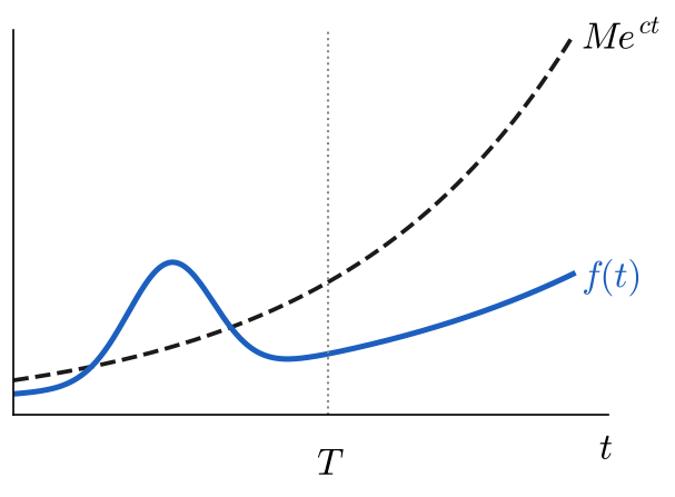
Graph of a function $f(t)$ (drawn thicker, in blue) and the dashed exponential curve $M{e}^{ct}$. Near $t=0$ the graph of $f$ has a bump that rises above the exponential, but for every $t>T$ the graph of $f$ stays below $M{e}^{ct}$.

Theorem: Sufficient Conditions for Existence

If $f$ is piecewise continuous on $[0,\infty )$ and of exponential order, then $ℒ\{f(t)\}$ exists for $s>c$.

Proof

$f$ is of exponential order, so there are constants $c,M>0,T>0$ such that $|f(t)|\le M{e}^{ct}$ for $t>T$. Split the integral at $T$:

$${\displaystyle ℒ\{f(t)\}={\int }_0^T{e}^{-st}f(t)dt+{\int }_T^{\infty }{e}^{-st}f(t)dt=I_1+I_2}$$

$I_1$ exists because $f$ is piecewise continuous (and the interval $[0,T]$ is finite). For $I_2$, use the bound on $|f(t)|$:

$${\displaystyle \begin{array}{cc}\hfill {\displaystyle |I_2|}& {\displaystyle \le {\int }_T^{\infty }{e}^{-st}|f(t)|dt\le M{\int }_T^{\infty }{e}^{-st}{e}^{ct}dt}\hfill \\ \hfill {\displaystyle }& {\displaystyle =M{\int }_T^{\infty }{e}^{-(s-c)t}dt={M\frac{e^{-(s-c)t}}{-(s-c)}|}_T^{\infty }}\hfill \\ \hfill {\displaystyle }& {\displaystyle =0+\frac{M}{s-c}{e}^{-(s-c)T},}\hfill \end{array}}$$

which is finite if $s>c$. $I_1$ converges and $I_2$ converges, so $I=I_1+I_2$ converges. ✓

“Sufficient” is a guarantee. The conditions given are not necessary conditions. That is, in some cases, $f$ is not of exponential order or not piecewise continuous, but $ℒ\{f(t)\}$ exists.

Theorem: Behavior of F(s) as s → ∞

If $f$ is piecewise continuous on $[0,\infty )$ and of exponential order and $F(s)=ℒ\{f(t)\}$, then ${\displaystyle \underset{s\to \infty }{lim}F(s)=0}$.

Proof

$f$ is of exponential order, so there exist $\gamma ,M_1>0,T>0$ such that $|f(t)|\le M_1{e}^{\gamma t}$ for $t>T$. ($\gamma$ is the Greek letter gamma.)

$f$ is piecewise continuous, so $f$ is bounded on $0\le t\le T$: $|f(t)|\le M_2=M_2{e}^{0t}$.

Let $M=max\{M_1,M_2\}$ and $c=max\{\gamma ,0\}$, so $|f(t)|\le M{e}^{ct}$ for all $t\ge 0$. Then

$${\displaystyle \begin{array}{cc}\hfill {\displaystyle |F(s)|}& {\displaystyle \le {\int }_0^{\infty }{e}^{-st}|f(t)|dt}\hfill \\ \hfill {\displaystyle }& {\displaystyle \le M{\int }_0^{\infty }{e}^{-st}{e}^{ct}dt=\frac{M}{s-c}}\hfill \end{array}}$$

for $s>c$. As $s\to \infty$, ${\displaystyle \frac{M}{s-c}\to 0}$, so $|F(s)|\to 0$; that is, $ℒ\{f(t)\}=F(s)\to 0$.

7.1d

Example

Use Definition 7.1.1 to find $ℒ\{f(t)\}$.

$$f(t)=\{\begin{array}{cc}{\displaystyle 2t+1,}\hfill & {\displaystyle 0\le t<1}\hfill \\ {\displaystyle 0,}\hfill & {\displaystyle t\ge 1}\hfill \end{array}$$

Solution

Split the integral where the formula changes: on [0, 1) the function is 2t + 1, and for t ≥ 1 it is 0.

$${\displaystyle ℒ\{f(t)\}={\int }_0^{\infty }{e}^{-st}f(t)dt={\int }_0^1(2t+1)e^{-st}dt+{\int }_1^{\infty }0dt}$$

The second integral is 0. Integrate the first by parts with $u=2t+1$, $dv=e^{-st}dt$, so $du=2dt$, ${\displaystyle v=-\frac{1}{s}{e}^{-st}}$:

$${\displaystyle \begin{array}{cc}\hfill {\displaystyle ℒ\{f(t)\}}& {\displaystyle ={-\frac{2t+1}{s{e}^{st}}|}_0^1+{\int }_0^1\frac{2}{s}{e}^{-st}dt}\hfill \\ \hfill {\displaystyle }& {\displaystyle =-\frac{3}{s{e}^s}+\frac{1}{s}-{\frac{2}{s^2{e}^{st}}|}_0^1}\hfill \\ \hfill {\displaystyle }& {\displaystyle =-\frac{3}{s{e}^s}+\frac{1}{s}-\frac{2}{s^2{e}^s}+\frac{2}{s^2}}\hfill \\ \hfill {\displaystyle }& {\displaystyle =\frac{1}{s}(1-3e^{-s})+\frac{2}{s^2}(1-e^{-s})}\hfill \end{array}}$$

Example

Use Definition 7.1.1 to find $ℒ\{f(t)\}$.

$f(t)=e^{-2t-5}$

Solution

$${\displaystyle \begin{array}{cc}\hfill {\displaystyle ℒ\left\{e^{-2t-5}\right\}}& {\displaystyle ={\int }_0^{\infty }{e}^{-st}{e}^{-2t-5}dt=e^{-5}{\int }_0^{\infty }{e}^{-(s+2)t}dt}\hfill \\ \hfill {\displaystyle }& {\displaystyle ={e^{-5}\frac{1}{-(s+2)e^{(s+2)t}}|}_0^{\infty }}\hfill \\ \hfill {\displaystyle }& {\displaystyle =e^{-5}\left(\frac{1}{s+2}\right)=\frac{e^{-5}}{s+2},s>-2}\hfill \end{array}}$$

The factor $e^{-5}$ is a constant, so it comes out of the integral. The value at the upper limit is 0 when $s+2>0$, that is, $s>-2$.

Example

Use Theorem 7.1.1 to find $ℒ\{f(t)\}$.

$f(t)=t^2-e^{-9t}+5$

Solution

By linearity, then parts (b) with $n=2$, (c) with $a=-9$, and (a):

$${\displaystyle \begin{array}{cc}\hfill {\displaystyle ℒ\{t^2-e^{-9t}+5\}}& {\displaystyle =ℒ\left\{t^2\right\}-ℒ\left\{e^{-9t}\right\}+5ℒ\left\{1\right\}}\hfill \\ \hfill {\displaystyle }& {\displaystyle =\frac{2}{s^3}-\frac{1}{s+9}+\frac{5}{s}}\hfill \end{array}}$$

$f(t)={\cos }^{2}t$

Solution

${\cos }^{2}t$ is not in the table, so first use the identity ${\cos }^{2}t=\frac{1}{2}(1+\cos 2t)$:

$${\displaystyle {\cos }^{2}t=\frac{1}{2}(1+\cos 2t)=\frac{1}{2}+\frac{1}{2}\cos 2t}$$

Now use parts (a) and (e) with $k=2$:

$${\displaystyle ℒ\{{\cos }^{2}t\}=\frac{1}{2s}+\frac{s}{2(s^2+4)}}$$