← Back to Math 055

3.2 Nonlinear Models: Class Notes

3.2a

Logistic growth

$${\displaystyle \frac{dP}{dt}=P(a-bP)=aP-b{P}^2}$$

This model is used with large populations, or when environmental factors inhibit growth.

Note: $-b{P}^2$ ($b>0$) is called an inhibition term or a competition term.

Justification for the model:

$${\displaystyle \frac{dP/dt}{P}=k}$$

is a constant relative growth rate (Section 3.1).

$${\displaystyle \frac{dP/dt}{P}=f(P)}$$

is a variable growth rate that still depends on the population.

If $K$ is the carrying capacity for the population (the maximum population), then $f(K)=0$. If we let $f(0)=r$, then in the simplest case $f$ is linear:

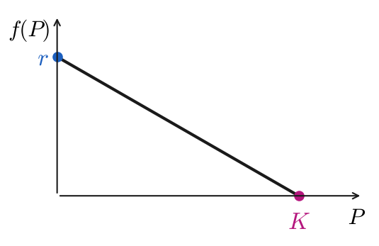
The simplest case: $f(P)$ is linear, with $f(0)=r$ (vertical intercept) and $f(K)=0$ (horizontal intercept at the carrying capacity).

$${\displaystyle f(P)=r-\frac{r}{K}P}$$

Then

$${\displaystyle \frac{dP}{dt}=P(r-\frac{r}{K}P).}$$

Relabeling gives ${\displaystyle \frac{dP}{dt}=P(a-bP)}$. Note: ${\displaystyle K=\frac{a}{b}}$ is the carrying capacity.

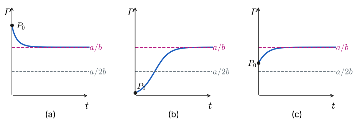
Logistic curves for different initial conditions. Each approaches the horizontal asymptote $P=a/b$. (a) $P_0>a/b$: $P$ decreases toward $a/b$. (b) $P_0<a/2b$: an S-shaped curve that increases, changing concavity where it crosses $P=a/2b$. (c) $a/2b<P_0<a/b$: $P$ increases toward $a/b$, concave down.

3.2b

Modified logistic growth

$${\displaystyle \frac{dP}{dt}=P(a-bP)\pm h}$$

$+h$: rate of restocking; $-h$: rate of harvesting.

Example

(a) If a constant number $h$ of fish are harvested from a fishery per unit time, then a model for the population $P(t)$ of the fishery at time $t$ is given by ${\displaystyle \frac{dP}{dt}=P(a-bP)-h,P(0)=P_0}$, where $a$, $b$, $h$, and $P_0$ are positive constants. Suppose $a=5$, $b=1$, and $h=4$. Since the DE is autonomous, use the phase portrait concept of Section 2.1 to sketch representative solution curves corresponding to the cases $P_0>4$, $1<P_0<4$, and $0<P_0<1$. Determine the long-term behavior of the population in each case.

Solution to (a)

$${\displaystyle \frac{dP}{dt}=P(5-P)-4=-P^2+5P-4=-(P^2-5P+4)=-(P-4)(P-1)}$$

The critical points are $P=1$ and $P=4$ (equilibrium solutions).

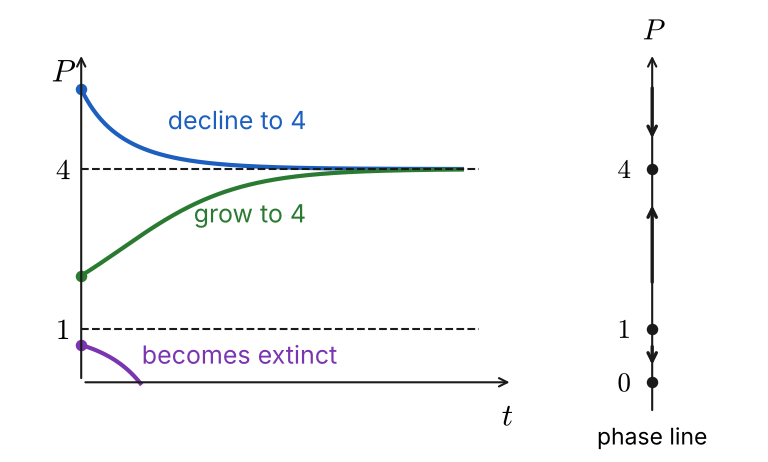
Phase line: $dP/dt<0$ (arrow down) for $P>4$, $dP/dt>0$ (arrow up) for $1<P<4$, and $dP/dt<0$ (arrow down) for $P<1$. Representative solution curves: starting above 4, $P$ declines to 4; starting between 1 and 4, $P$ grows to 4; starting between 0 and 1, $P$ decreases and reaches 0 (extinction).

If $P_0>4$, $P$ will decline to 4.

If $1<P_0<4$, $P$ will increase to 4.

If $0<P_0<1$, the population will go extinct.

(Values $P<0$ on the phase line don’t apply to populations.)

(b) Solve the IVP in part (a). Verify the results of your phase portrait in part (a) by using a graphing utility to plot the graph of $P(t)$ with an initial condition taken from each of the three intervals given.

Solution to (b)

$${\displaystyle \frac{dP}{dt}=-(P-1)(P-4),P(0)=P_0}$$

Separate the variables:

$${\displaystyle \frac{dP}{(P-1)(P-4)}=-dt}$$

Partial fractions (PFD):

$${\displaystyle \int (\frac{1/3}{P-4}-\frac{1/3}{P-1})dP=\int (-1)dt}$$

$${\displaystyle \frac{1}{3}\ln \left|\frac{P-4}{P-1}\right|=-t+C_1}$$

$${\displaystyle \frac{P-4}{P-1}=C{e}^{-3t}}$$

Apply $P(0)=P_0$:

$${\displaystyle C=\frac{P_0-4}{P_0-1}}$$

Solve for $P$: $P-4=C{e}^{-3t}(P-1)$, so $P(1-C{e}^{-3t})=4-C{e}^{-3t}$.

$${\displaystyle P(t)=\frac{4-C{e}^{-3t}}{1-C{e}^{-3t}}=\frac{4-\frac{P_0-4}{P_0-1}{e}^{-3t}}{1-\frac{P_0-4}{P_0-1}{e}^{-3t}}}$$

Multiply the top and bottom by $P_0-1$:

Equivalently (multiplying the top and bottom by $-e^{3t}$),

$${\displaystyle P(t)=\frac{P_0-4-4(P_0-1)e^{3t}}{P_0-4-(P_0-1)e^{3t}}.}$$

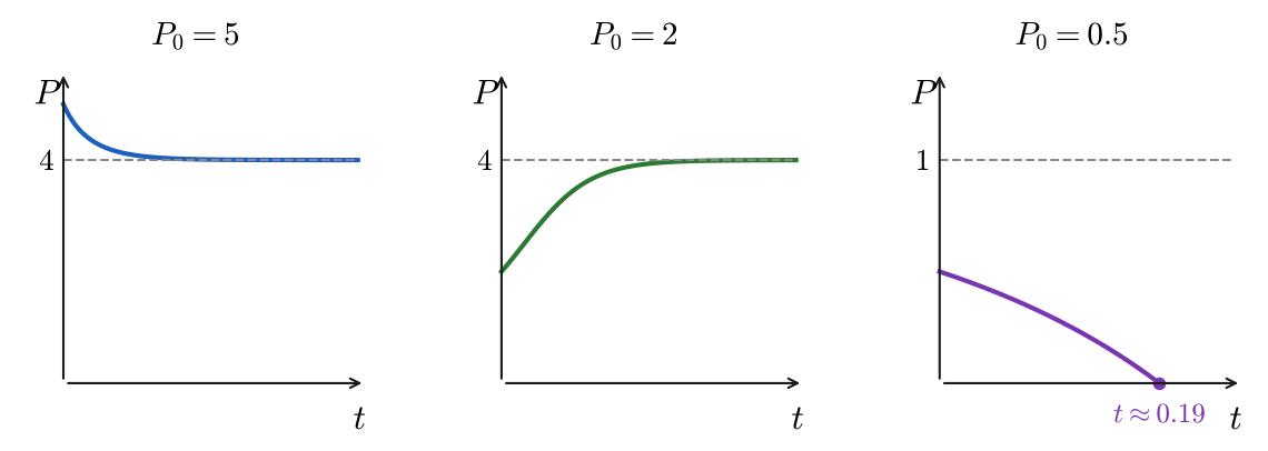
Graphs of the solution $P(t)$ from part (b). With $P_0=5$, $P$ decreases to 4. With $P_0=2$, $P$ increases to 4. With $P_0=0.5$, $P$ decreases and reaches 0 at about $t\approx 0.19$ (this graph uses a shorter time scale, with $P=1$ dashed).

The graphs agree with the phase portrait in part (a).

(c) Use the information in parts (a) and (b) to determine whether the fishery population becomes extinct in finite time. If so, find that time.

Solution to (c)

Does $P=0$? That happens when the numerator is 0:

$${\displaystyle 4(P_0-1)-(P_0-4)e^{-3t}=0\Rightarrow e^{-3t}=\frac{4(P_0-1)}{P_0-4}}$$

From part (a), this happens only when $0<P_0<1$ (then the fraction is between 0 and 1, so $t>0$): the population becomes extinct in finite time.

3.2c

Second-order chemical reaction

$${\displaystyle \frac{dX}{dt}=k(\alpha -X)(\beta -X),}$$

where ${\displaystyle \alpha =\frac{a(M+N)}{M}}$ and ${\displaystyle \beta =\frac{b(M+N)}{N}}$,
$a$ = # grams of chemical $A$,
$b$ = # grams of chemical $B$, and
$X(t)$ is grams of $C$, formed from $M$ parts of $A$ and $N$ parts of $B$

When $M$ parts of $A$ combine with $N$ parts of $B$, they form $M+N$ parts of $C$. So of the $X$ grams of $C$, ${\displaystyle \frac{M}{M+N}X}$ grams came from $A$ and ${\displaystyle \frac{N}{M+N}X}$ grams came from $B$.

For example, if 3 parts of $A$ combine with 2 parts of $B$, then $3+2=5$ parts of $C$ form, and ${\displaystyle \frac{3}{5}}$ of $C$ comes from $A$ and ${\displaystyle \frac{2}{5}}$ from $B$.

The rate is proportional to the amounts of $A$ and $B$ remaining:

$${\displaystyle \frac{dX}{dt}=k_1(a-\frac{M}{M+N}X)(b-\frac{N}{M+N}X)}$$

Factoring ${\displaystyle \frac{M}{M+N}}$ and ${\displaystyle \frac{N}{M+N}}$ out of the two factors gives

$${\displaystyle \frac{dX}{dt}=k(\alpha -X)(\beta -X),\alpha =\frac{a(M+N)}{M},\beta =\frac{b(M+N)}{N}.}$$

Example

Two chemicals $A$ and $B$ are combined to form a chemical $C$. The rate, or velocity, of the reaction is proportional to the product of the instantaneous amounts of $A$ and $B$ not converted to chemical $C$. Initially, there are 80 grams of $A$ and 50 grams of $B$, and for each gram of $B$, 2 grams of $A$ is used. It is observed that 10 grams of $C$ is formed in 10 minutes. How much is formed in 40 minutes? What is the limiting amount of $C$ after a long time? How much of chemicals $A$ and $B$ remains after a long time?

Solution

$${\displaystyle \frac{dX}{dt}=k(\alpha -X)(\beta -X)}$$

Here $a=80$, $b=50$, and (2 grams of $A$ for each gram of $B$) $M=2$, $N=1$.

$${\displaystyle \alpha =\frac{80(3)}{2}=120,\beta =\frac{50(3)}{1}=150}$$

$${\displaystyle \frac{dX}{dt}=k(120-X)(150-X)\Rightarrow \frac{dX}{(120-X)(150-X)}=kdt}$$

Partial fractions (PFD):

$${\displaystyle \int (\frac{1/30}{120-X}-\frac{1/30}{150-X})dX=\int kdt}$$

$${\displaystyle \frac{1}{30}\ln \left|\frac{150-X}{120-X}\right|=kt+C}$$

$${\displaystyle \ln \left|\frac{150-X}{120-X}\right|=k_{1}t+C_1}$$

Use $X(0)=0$: $C_1=\ln \frac{5}{4}$, so

$${\displaystyle \frac{150-X}{120-X}=\frac{5}{4}{e}^{k_{1}t}.}$$

Use $X(10)=10$: ${\displaystyle \frac{140}{110}=\frac{5}{4}{e}^{10k_1}}$, so ${\displaystyle e^{10k_1}=\frac{56}{55}}$ and

$${\displaystyle k_1=\frac{1}{10}\ln \frac{56}{55}\approx 0.0018.}$$

Solve for $X$: $4(150-X)=5e^{k_{1}t}(120-X)$, so

$${\displaystyle X(t)=\frac{600(e^{0.0018t}-1)}{5e^{0.0018t}-4}=\frac{600(1-e^{-0.0018t})}{5-4e^{-0.0018t}}.}$$

At 40 minutes:

After a long time ($e^{-0.0018t}\to 0$):

Initially there are 80 g of $A$ and 50 g of $B$. The 120 g of $C$ use 80 g of $A$ and 40 g of $B$, so 0 g of $A$ and 10 g of $B$ are left over: $A$ is the limiting factor.