← Back to Math 055

2.6 A Numerical Method (Euler’s Method): Class Notes

2.6a

Recall the equation of the tangent line of the solution curve for the differential equation $y\prime =f(x,y),y(x_0)=y_0$ is $y=y_0+f(x_0,y_0)(x-x_0)$.

Tip: This is the point-slope form $y-y_1=m(x-x_1)$, with slope $m=f(x_0,y_0)$.

Definition

This is known as the linearization of $f$ at $(x_0,y_0)$.

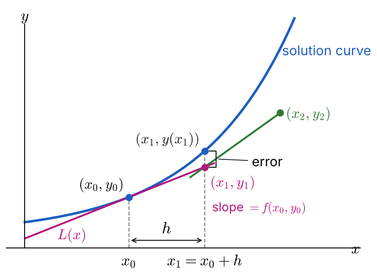
A solution curve of $y\prime =f(x,y)$ passes through $(x_0,y_0)$. Its tangent line $L(x)$ there has slope $f(x_0,y_0)$. Moving a distance $h$ to the right, to $x_1=x_0+h$, the tangent line reaches the point $(x_1,y_1)$, while the curve is at $(x_1,y(x_1))$; the vertical gap between them is the error. From $(x_1,y_1)$, a second line segment with slope $f(x_1,y_1)$ leads to $(x_2,y_2)$.

If we consider $(x_1,y_1)$ with $x$-value $x_1=x_0+h$ (a small distance $h$ to the right of $x_0$), we have

$$y_1=y_0+hf(x_0,y_0).$$

$(x_1,y_1)$ is an approximation to $(x_1,y(x_1))$, which is on the solution curve. Using $(x_1,y_1)$ and the slope given by $y\prime =f(x,y)$ at that point, we get

$$y_2=y_1+hf(x_1,y_1)$$

and $(x_2,y_2)$, where $x_2=x_1+h=x_0+2h$.

This process continues, and we can generalize the results:

$$\begin{array}{cc}\hfill {\displaystyle x_{n+1}}& {\displaystyle =x_n+h}\hfill \\ \hfill {\displaystyle y_{n+1}}& {\displaystyle =y_n+hf(x_n,y_n),n=0,1,2,\dots }\hfill \end{array}$$

Example

Use Euler’s method to obtain a four-decimal approximation of the indicated value. Carry out the recursion by hand, first using $h=0.1$ and then using $h=0.05$.

$$y\prime =x+y^2,y(0)=0;y(0.2)$$

Solution

Here $f(x,y)=x+y^2$ and $(x_0,y_0)=(0,0)$.

$h=0.1$: Each new $y$-value is the previous $y$-value plus $h$ times $f$ at the previous point.

$$\begin{array}{cc}\hfill {\displaystyle x_1=0.1,y(0.1)\approx y_1}& {\displaystyle =0+0.1(0+0^2)=0}\hfill \\ \hfill {\displaystyle x_2=0.2,y(0.2)\approx y_2}& {\displaystyle =0+0.1(0.1+0^2)=0.01}\hfill \end{array}$$

$h=0.05$: Start again from $x_0=0,y_0=0$.

$$\begin{array}{cc}\hfill {\displaystyle x_1=0.05,y(0.05)\approx y_1}& {\displaystyle =0+0.05(0+0^2)=0}\hfill \\ \hfill {\displaystyle x_2=0.1,y(0.1)\approx y_2}& {\displaystyle =0+0.05(0.05+0^2)=0.0025}\hfill \\ \hfill {\displaystyle x_3=0.15,y(0.15)\approx y_3}& {\displaystyle =0.0025+0.05(0.1+{0.0025}^2)\approx 0.0075}\hfill \\ \hfill {\displaystyle x_4=0.2,y(0.2)\approx y_4}& {\displaystyle =0.0075+0.05(0.15+{0.0075}^2)\approx 0.0150}\hfill \end{array}$$

2.6b

Example

Use Euler’s method to obtain a four-decimal approximation of the indicated value. First use $h=0.1$ and then use $h=0.05$. Find an explicit solution for each initial-value problem and then construct a table displaying estimated value, actual value, absolute error, and percentage relative error.

$$y\prime =2xy,y(1)=1;y(1.5)$$

Solution

Analytic solution. The DE is separable:

$${\displaystyle \frac{dy}{y}=2xdx\Rightarrow \ln |y|=x^2+c}$$

With $y(1)=1$: $0=1+c$, so $c=-1$ and $y=e^{x^2-1}$.

The DE is also linear: $y\prime -2xy=0$ has $\mu =e^{-x^2}$, so

$${\displaystyle \frac{d}{dx}\left(e^{-x^2}y\right)=0\Rightarrow e^{-x^2}y=c\Rightarrow y=c{e}^{x^2}.}$$

With $y(1)=1$: $1=ce$, so $c=e^{-1}$ and $y=e^{x^2}{e}^{-1}=e^{x^2-1}$.

Euler’s method. Here $f(x,y)=2xy$, and $y_{n+1}=y_n+h·2x_n{y}_n$. The tables list each step with the actual value $y(x_n)=e^{x_n^2-1}$, the absolute error $|y(x_n)-y_n|$, and the percentage relative error

$${\displaystyle \frac{|y(x_n)-y_n|}{y(x_n)}·100\%.}$$

For $h=0.1$, $y(1.5)\approx 2.9278$. For $h=0.05$, $y(1.5)\approx 3.1733$. The actual value is $y(1.5)=e^{1.25}\approx 3.4903$.

When $h$ is cut in half, the error is cut roughly in half (at $x=1.5$: $0.5625\to 0.3171$). The error is $O(h)$.